
Survival Analysis
1.Survival Analysis Basics
Basic concept
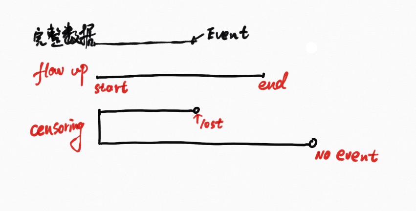
Censoring:right censoring
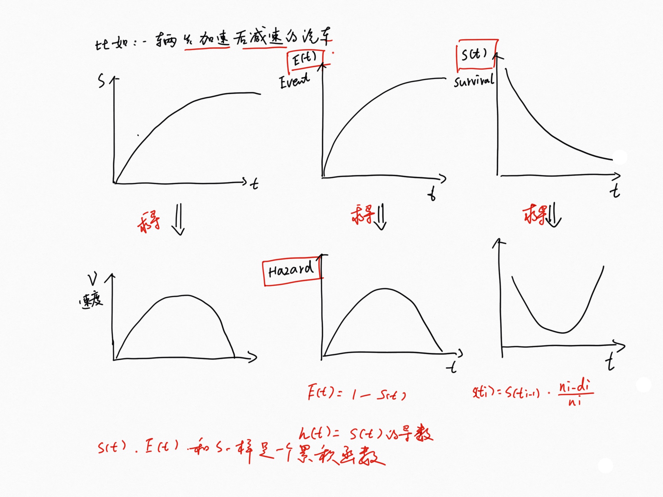
Survival and hazard functions
Log-rank test: Kaplan-Meier survival estimate
null hypothesis is that there is no difference in survival between the two groups
- Non-parametric test , so no assumptions about the survival distributions
- Log rank statistic is approximately distributed as a chi-square test statistic.
Survival analysis in R
#data
library("survival")
library("survminer")
data("lung")
#survival fit
fit <- survfit(Surv(time, status) ~ sex, data = lung)
#summary
summary(fit)$table
## records n.max n.start events *rmean *se(rmean) median 0.95LCL
## sex=1 138 138 138 112 325.0663 22.59845 270 212
## sex=2 90 90 90 53 458.2757 33.78530 426 348
## 0.95UCL
## sex=1 310
## sex=2 550d <- data.frame(time = fit$time,
n.risk = fit$n.risk,
n.event = fit$n.event,
n.censor = fit$n.censor,
surv = fit$surv,
upper = fit$upper,
lower = fit$lower
)
head(d)## time n.risk n.event n.censor surv upper lower
## 1 11 138 3 0 0.9782609 1.0000000 0.9542301
## 2 12 135 1 0 0.9710145 0.9994124 0.9434235
## 3 13 134 2 0 0.9565217 0.9911586 0.9230952
## 4 15 132 1 0 0.9492754 0.9866017 0.9133612
## 5 26 131 1 0 0.9420290 0.9818365 0.9038355
## 6 30 130 1 0 0.9347826 0.9768989 0.8944820#Visualize survival curves
ggsurvplot(
fit, # survfit object with calculated statistics.
pval = TRUE, # show p-value of log-rank test.
conf.int = TRUE, # show confidence intervals for
# point estimaes of survival curves.
conf.int.style = "step", # customize style of confidence intervals
xlab = "Time in days", # customize X axis label.
break.time.by = 200, # break X axis in time intervals by 200.
ggtheme = theme_light(), # customize plot and risk table with a theme.
risk.table = "abs_pct", # absolute number and percentage at risk.
risk.table.y.text.col = T,# colour risk table text annotations.
risk.table.y.text = FALSE,# show bars instead of names in text annotations
# in legend of risk table.
ncensor.plot = TRUE, # plot the number of censored subjects at time t
surv.median.line = "hv", # add the median survival pointer.
legend.labs =
c("Male", "Female"), # change legend labels.
palette =
c("#E7B800", "#2E9FDF") # custom color palettes.
)
ggsurvplot(fit,
conf.int = TRUE,
risk.table.col = "strata",
ggtheme = theme_bw(),
palette = c("#E7B800", "#2E9FDF"),
fun = "cumhaz")
#Log-rank test
surv_diff <- survdiff(Surv(time, status) ~ sex, data = lung)
surv_diff
## Call:
## survdiff(formula = Surv(time, status) ~ sex, data = lung)
##
## N Observed Expected (O-E)^2/E (O-E)^2/V
## sex=1 138 112 91.6 4.55 10.3
## sex=2 90 53 73.4 5.68 10.3
##
## Chisq= 10.3 on 1 degrees of freedom, p= 0.0012.Cox Proportional Hazards Model
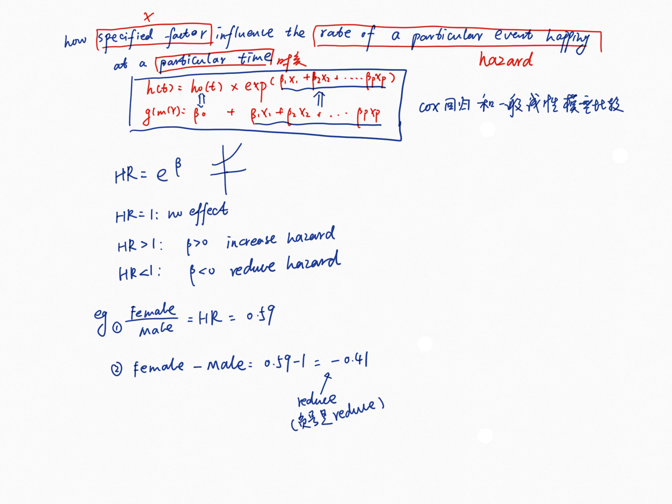
Concept
- Kaplan-Meier curves and log-rank tests - are examples of univariate analysis.
- Additionally, Kaplan-Meier curves and logrank tests are useful only when the predictor variable is categorical (e.g.: treatment A vs treatment B; males vs females). They don’t work easily for quantitative predictors such as gene expression, weight, or age.
- Cox proportional hazards regression analysis, which works for both quantitative predictor variables and for categorical variables.
Compute the Cox model in R
#data

#fit
res.cox <- coxph(Surv(time, status) ~ sex, data = lung)
#summary
summary(res.cox)
## Call:
## coxph(formula = Surv(time, status) ~ sex, data = lung)
##
## n= 228, number of events= 165
##
## coef exp(coef) se(coef) z Pr(>|z|)
## sex -0.5310 0.5880 0.1672 -3.176 0.00149 **
## ---
## Signif. codes: 0 '***' 0.001 '**' 0.01 '*' 0.05 '.' 0.1 ' ' 1
##
## exp(coef) exp(-coef) lower .95 upper .95
## sex 0.588 1.701 0.4237 0.816
##
## Concordance= 0.579 (se = 0.022 )
## Rsquare= 0.046 (max possible= 0.999 )
## Likelihood ratio test= 10.63 on 1 df, p=0.001
## Wald test = 10.09 on 1 df, p=0.001
## Score (logrank) test = 10.33 on 1 df, p=0.001covariates <- c("age", "sex", "ph.karno", "ph.ecog", "wt.loss")
univ_formulas <- sapply(covariates,
function(x) as.formula(paste('Surv(time, status)~', x)))
univ_models <- lapply( univ_formulas, function(x){coxph(x, data = lung)})
# Extract data
univ_results <- lapply(univ_models,
function(x){
x <- summary(x)
p.value<-signif(x$wald["pvalue"], digits=2)
wald.test<-signif(x$wald["test"], digits=2)
beta<-signif(x$coef[1], digits=2);#coeficient beta
HR <-signif(x$coef[2], digits=2);#exp(beta)
HR.confint.lower <- signif(x$conf.int[,"lower .95"], 2)
HR.confint.upper <- signif(x$conf.int[,"upper .95"],2)
HR <- paste0(HR, " (",
HR.confint.lower, "-", HR.confint.upper, ")")
res<-c(beta, HR, wald.test, p.value)
names(res)<-c("beta", "HR (95% CI for HR)", "wald.test",
"p.value")
return(res)
#return(exp(cbind(coef(x),confint(x))))
})
res <- t(as.data.frame(univ_results, check.names = FALSE))
as.data.frame(res)## beta HR (95% CI for HR) wald.test p.value
## age 0.019 1 (1-1) 4.1 0.042
## sex -0.53 0.59 (0.42-0.82) 10 0.0015
## ph.karno -0.016 0.98 (0.97-1) 7.9 0.005
## ph.ecog 0.48 1.6 (1.3-2) 18 2.7e-05
## wt.loss 0.0013 1 (0.99-1) 0.05 0.83Multivariate Cox regression analysis
#fit
res.cox <- coxph(Surv(time, status) ~ age + sex + ph.ecog, data =  lung)
summary(res.cox)
## Call:
## coxph(formula = Surv(time, status) ~ age + sex + ph.ecog, data = lung)
##
## n= 227, number of events= 164
## (1 observation deleted due to missingness)
##
## coef exp(coef) se(coef) z Pr(>|z|)
## age 0.011067 1.011128 0.009267 1.194 0.232416
## sex -0.552612 0.575445 0.167739 -3.294 0.000986 ***
## ph.ecog 0.463728 1.589991 0.113577 4.083 4.45e-05 ***
## ---
## Signif. codes: 0 '***' 0.001 '**' 0.01 '*' 0.05 '.' 0.1 ' ' 1
##
## exp(coef) exp(-coef) lower .95 upper .95
## age 1.0111 0.9890 0.9929 1.0297
## sex 0.5754 1.7378 0.4142 0.7994
## ph.ecog 1.5900 0.6289 1.2727 1.9864
##
## Concordance= 0.637 (se = 0.026 )
## Rsquare= 0.126 (max possible= 0.999 )
## Likelihood ratio test= 30.5 on 3 df, p=1e-06
## Wald test = 29.93 on 3 df, p=1e-06
## Score (logrank) test = 30.5 on 3 df, p=1e-06sex_df <- with(lung,
data.frame(sex = c(1, 2),
age = rep(mean(age, na.rm = TRUE), 2),
ph.ecog = c(1, 1)
)
)
sex_df## sex age ph.ecog
## 1 1 62.44737 1
## 2 2 62.44737 1# Survival curves
fit <- survfit(res.cox, newdata = sex_df)
ggsurvplot(fit, data=lung, conf.int = TRUE, legend.labs=c("Sex=1", "Sex=2"),
ggtheme = theme_minimal())
3.Cox Model Assumptions
1. the Schoenfeld residuals are independent of time, non-significant relationship between residuals and time
#From the output down, the test is not statistically significant for each of the covariates
res.cox <- coxph(Surv(time, status) ~ age + sex + wt.loss, data =  lung)
res.cox
## Call:
## coxph(formula = Surv(time, status) ~ age + sex + wt.loss, data = lung)
##
## coef exp(coef) se(coef) z p
## age 0.02009 1.02029 0.00966 2.08 0.0377
## sex -0.52103 0.59391 0.17435 -2.99 0.0028
## wt.loss 0.00076 1.00076 0.00619 0.12 0.9024
##
## Likelihood ratio test=14.67 on 3 df, p=0.002
## n= 214, number of events= 152
## (14 observations deleted due to missingness)test.ph <- cox.zph(res.cox)
test.ph## rho chisq p
## age -0.0483 0.378 0.538
## sex 0.1265 2.349 0.125
## wt.loss 0.0126 0.024 0.877
## GLOBAL NA 2.846 0.416ggcoxzph(test.ph)
2. influential observations
hat(y) - y 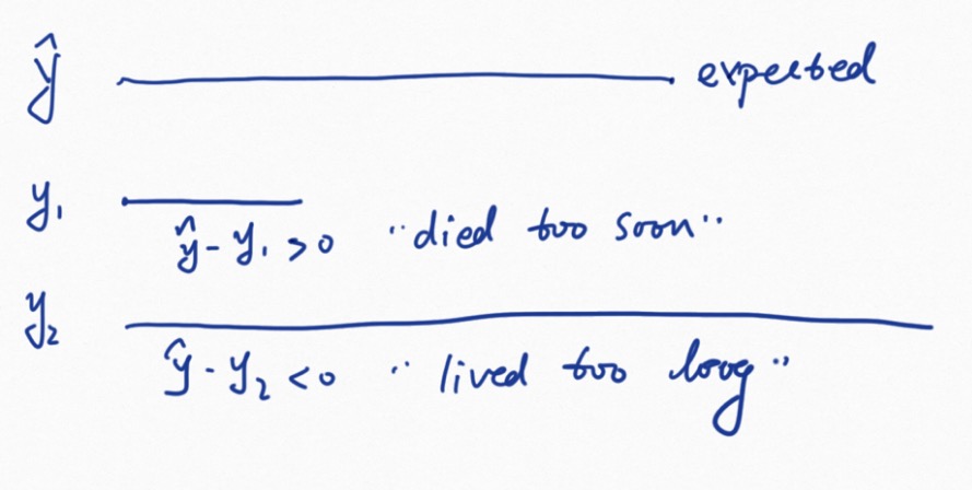 1. Positive values correspond to individuals that “died too soon” compared to expected survival times. 2. Negative values correspond to individual that “lived too long”. 3. Very large or small values are outliers, which are poorly predicted by the model.
#type: the type of residuals to present on Y axis. Allowed values include one of c(“martingale”, “deviance”, “score”, “schoenfeld”, “dfbeta”, “dfbetas”, “scaledsch”, “partial”)
ggcoxdiagnostics(res.cox, type = "dfbeta",
                 linear.predictions = FALSE, ggtheme = theme_bw())
ggcoxdiagnostics(res.cox, type = "deviance",
                 linear.predictions = FALSE, ggtheme = theme_bw())
3.non linearity
we assume that continuous covariates have a linear form. However, this assumption should be checked Martingale residuals may present any value in the range (-INF, +1) : 1. A value of martinguale residuals near 1 represents individuals that “died too soon”, 2. and large negative values correspond to individuals that “lived too long”.
The function ggcoxfunctional() displays graphs of continuous covariates against martingale residuals of null cox proportional hazards model. This might help to properly choose the functional form of continuous variable in the Cox model . Fitted lines with lowess function should be linear to satisfy the Cox proportional hazards model assumptions.
#It appears that, nonlinearity is slightly here.
ggcoxfunctional(Surv(time, status) ~ age + log(age) + sqrt(age), data = lung)
#比较 变量age 在 线性age 和非线性 log(age) or sqrt(age) 下 残差分布模式图,基本一致,所以线性假设满足